As we discussed today in class and as mentioned by Laurent in his post, adding gaussian noise is important to prevent convergence to a constant. In my last post, I found this kind of behaviour which results in a flatline.
Recall Laurent’s post:

where 
The estimator of the variance is the mean square error (MSE):
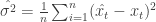
where 
Compared to my previous post, I only had to modify the output of the neural network to generate speech. Concretely, I sampled from a gaussian distribution which mean equals to the output of the neural network and which variance equals to the MSE of the training examples. You will find that in the same mlp.py script (go to line 380).
Here are the results (note that I used the same previous hyperparameters):

Learning curve. Note that I normalized the samples by dividing them by 560 which is roughly the standard error.

Generation of the acoustic based on a NN trained for 100 epochs. It starts at sample 2500 of the SX397.WAV and then generates the next 30 000 samples.
For those interested in listening the resulting generated speech (in case of the audio player doesn’t work, here is the link to the .wav file):
https://dl.dropboxusercontent.com/u/43075537/generated_data.wav%20In conclusion it doesn’t sound like Georges Brassens but it does break the undesired behaviour described above!

This is a very interesting result! I analysed the spectrum of your model’s output file and it looks a lot like speech in average should look (high energy in low frequency components, with a 10 dB/octave decay), which probably means the model was capable of capturing this aspect of speech’s distribution.